Traveling Dots, Parabolas, and Elegant Math

Toward the end of last week, I read a description a variation on a paper-folding strategy to create parabolas.  Paraphrased, it said:

1. On a piece of wax paper, use a pen to draw a line near one edge.  (I used a Sharpie on regular copy paper and got enough ink bleed that I’m convinced any standard copy or notebook paper will do.  I don’t think the expense of wax paper is required!)
2. All along the line, place additional dots 0.5 to 1 inch apart.
3. Finally, draw a point F between 0.5 and 2 inches from the line roughly along the midline of the paper toward the center of the paper.
4. Fold the paper over so one of the dots on line is on tope of point F.  Crease the paper along the fold and open the paper back up.
5. Repeat step 4 for every dot you drew in step 2.
6. All of the creases from steps 4 & 5 outline a curve.  Trace that curve to see a parabola.

I’d seen and done this before, I had too passively trusted that the procedure must have been true just because the resulting curve “looked like a parabola.”  I read the proof some time ago, but I consumed it too quickly and didn’t remember it when I was read the above procedure.  I shamefully admitted to myself that I was doing exactly what we insist our students NEVER do–blindly accepting a “truth” based on its appearance.  So I spent part of that afternoon thinking about how to understand completely what was going on here.

What follows is the chronological redevelopment of my chain of reasoning for this activity, hopefully showing others that the prettiest explanations rarely occur without effort, time, and refinement.  At the end of this post, I offer what I think is an even smoother version of the activity, freed from some of what I consider overly structured instructions above.

CONIC DEFINITION AND WHAT WASN’T OBVIOUS TO ME

A parabola is the locus of points equidistant from a given  point (focus) and line (directrix).

What makes the parabola interesting, in my opinion, is the interplay between the distance from a line (always perpendicular to some point C on the directrix) and the focus point (theoretically could point in any direction like a radius from a circle center).

What initially bothered me about the paper folding approach last week was that it focused entirely on perpendicular bisectors of the Focus-to-C segment (using the image above).  It was not immediately obvious to me at all that perpendicular bisectors of the Focus-to-C segment were 100% logically equivalent to the parabola’s definition.

SIMILARITY ADVANTAGES AND PEDAGOGY

I think I had two major advantages approaching this.

1. I knew without a doubt that all parabolas are similar (there is a one-to-one mapping between every single point on any parabola and every single point on any other parabola), so I didn’t need to prove lots of cases.  Instead, I focused on the simplest version of a parabola (from my perspective), knowing that whatever I proved from that example was true for all parabolas.
2. I am quite comfortable with my algebra, geometry, and technology skills.  Being able to wield a wide range of powerful exploration tools means I’m rarely intimidated by problems–even those I don’t initially understand.  I have the patience to persevere through lots of data and explorations until I find patterns and eventually solutions.

I love to understand ideas from multiple perspectives, so I rarely quit with my initial solution.  Perseverance helps me re-phrase ideas and exploring them from alternative perspectives until I find prettier ways of understanding.

In my opinion, it is precisely this willingness to play, persevere, and explore that formalized education is broadly failing to instill in students and teachers.  “What if?” is the most brilliant question, and the one we sadly forget to ask often enough.

ALGEBRAIC PROOF

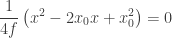
While I’m comfortable handling math in almost any representation, my mind most often jumps to algebraic perspectives first.  My first inclination was a coordinate proof.

PROOF 1:  As all parabolas are similar, it was enough to use a single, upward facing parabola with its vertex at the origin.  I placed the focus at , making the directrix the line .  If any point on the parabola was , then a point C on the directrix was at .

From the parabola’s definition, the distance from the focus to P was identical to the length of CP:

Squaring and combining common terms gives

But the construction above made lines (creases) on the perpendicular bisector of the focus-to-C segment.  This segment has midpoint and slope , so an equation for its perpendicular bisector is .

Finding the point of intersection of the perpendicular bisector with the parabola involves solving a system of equations.

So the only point where the line and parabola meet is at –the very same point named by the parabola’s definition.  QED

Proof 2:  All of this could have been brilliantly handled on a CAS to save time and avoid the manipulations.

Notice that the y-coordinate of the final solution line is the same from above.

MORE ELEGANT GEOMETRIC PROOFS

I had a proof, but the algebra seemed more than necessary.  Surely there was a cleaner approach.

In the image above, F is the focus, and I is a point on the parabola.  If D is the midpoint of , can I conclude , proving that the perpendicular bisector of always intersects the parabola?

PROOF 3:  The definition of the parabola gives , and the midpoint gives .  Because is self-congruent, by SSS, and corresponding parts make the supplementary , so both must be right angles.  QED

PROOF 4:  Nice enough, but it still felt a little complicated.  I put the problem away to have dinner with my daughters and when I came back, I was able to see the construction not as two congruent triangles, but as the single isosceles with base .  In isosceles triangles, altitudes and medians coincide, automatically making the perpendicular bisector of .  QED

Admittedly, Proof 4 ultimately relies on the results of Proof 3, but the higher-level isosceles connection felt much more elegant.  I was satisfied.

TWO DYNAMIC GEOMETRY SOFTWARE VARIATIONS

Thinking how I could prompt students along this path, I first considered a trace on the perpendicular lines from the initial procedure above (actually tangent lines to the parabola) using to trace the parabolas.  A video is below, and the Geogebra file is here.

http://vimeo.com/89759785

It is a lovely approach, and I particularly love the way the parabola appears as a digital form of “string art.”  Still, I think it requires some additional thinking for users to believe the approach really does adhere to the parabola’s definition.

I created a second version allowing users to set the location of the focus on the positive y-axis and using  a slider to determine the distances and constructs the parabola through the definition of the parabola.  [In the GeoGebra worksheet (here), you can turn on the hidden circle and lines to see how I constructed it.]  A video shows the symmetric points traced out as you drag the distance slider.

http://vimeo.com/89861149

A SIMPLIFIED PAPER PROCEDURE

Throughout this process, I realized that the location and spacing of the initial points on the directrix was irrelevant.  Creating the software versions of the problem helped me realize that if I could fold a point on the directrix to the focus, why not reverse the process and fold F to the directrix?  In fact, I could fold the paper so that F touched anywhere on the directrix and it would work.  So, here is the simplest version I could develop for the paper version.

1. Use a straightedge and a Sharpie or thin marker to draw a line near the edge of a piece of paper.
2. Place a point F roughly above the middle of the line toward the center of the paper.
3. Fold the paper over so point F is on the line from step 1 and crease the paper along the fold.
4. Open the paper back up and repeat step 3 several more times with F touching other parts of the step 1 line.
5. All of the creases from steps 3 & 4 outline a curve.  Trace that curve to see a parabola.

This procedure works because you can fold the focus onto the directrix anywhere you like and the resulting crease will be tangent to the parabola defined by the directrix and focus.  By allowing the focus to “Travel along the Directrix”, you create the parabola’s locus.  Quite elegant, I thought.

ADDITIONAL POSSIBLE QUESTIONS

As I was playing with the different ways to create the parabola and thinking about the interplay between the two distances in the parabola’s definition, I wondered about the potential positions of the distance segments.

1. What is the shortest length of segment CP and where could it be located at that length?  What is the longest length of segment CP and where could it be located at that length?
2. Obviously, point C can be anywhere along the directrix.  While the focus-to-P segment is theoretically free to rotate in any direction, the parabola definition makes that seem not practically possible.  So, through what size angle is the focus-to-P segment practically able to rotate?
3. Assuming a horizontal directrix, what is the maximum slope the focus-to-P segment can achieve?
4. Can you develop a single solution to questions 2 and 3 that doesn’t require any computations or constructions?

CONCLUSIONS

I fully realize that none of this is new mathematics, but I enjoyed the walk through pure mathematics and the enjoyment of developing ever simpler and more elegant solutions to the problem.  In the end, I now have a deeper and richer understanding of parabolas, and that was certainly worth the journey.

The Value of Counter-Intuition

Numberphile caused quite a stir when it posted a video explaining why

Doug Kuhlman recently posted a great follow-up Numberphile video explaining a broader perspective behind this sum.

It’s a great reminder that there are often different ways of thinking about problems, and sometimes we have to abandon tradition to discover deeper, more elegant connections.

For those deeply bothered by this summation result, the second video contains a lovely analogy to the “reality” of .  From one perspective, it is absolutely not acceptable to do something like square roots of negative numbers.  But by finding a way to conceptualize what such a thing would mean, we gain a far richer understanding of the very real numbers that forbade  in the first place as well as opening the doors to stunning mathematics far beyond the limitations of real numbers.

On the face of it, is obviously wrong within the context of real numbers only.  But the strange thing in physics and the Zeta function and other places is that just happens to work … every time.  Let’s not dismiss this out of hand.  It gives our students the wrong idea about mathematics, discovery, and learning.

There’s very clearly SOMETHING going on here.  It’s time to explore and learn something deeper.  And until then, we can revel in the awe of manipulations that logically shouldn’t work, but somehow they do.

May all of our students feel the awe of mathematical and scientific discovery.  And until the connections and understanding are firmly established, I hope we all can embrace the spirit, boldness, and fearless of Euler.

Midpoints, midpoints, everywhere!

I didn’t encounter the Quadrilateral Midpoint Theorem (QMT) until I had been teaching a few years.  Following is a minor variation on my approach to the QMT this year plus a fun way I leveraged the result to introduce similarity.

In case you haven’t heard of it, the surprisingly lovely QMT says that if you connect, in order, the midpoints of the four sides of a quadrilateral–any quadrilateral–even if the quadrilateral is concave or if its sides cross–the resulting figure will always be a parallelogram.

This is a cool and easy property to explore on any dynamic geometry software package (GeoGebra, TI-Nspire, Cabri, …).

SKETCH OF THE TRADITIONAL PROOF:  The proof is often established through triangle similarity:  Whenever you connect the midpoints of two sides of a triangle, the resulting segment will be parallel to and half the length of the triangle’s third side.  Draw either diagonal in the quadrilateral to create two triangles.  Connecting the midpoints of the other two sides of each triangle creates two congruent parallel sides, so the quadrilateral connecting all four midpoints must be a parallelogram.

NEW APPROACH THIS YEAR:  I hadn’t yet led my class into similarity, but having just introduced coordinate proofs, I tried an approach I’d never used before.  I assigned a coordinate proof of the QMT.  I knew the traditional approach existed, but I wanted them to practice their new technique.  From a lab in December, they already knew the result of the QMT, but they hadn’t proved it.

PART I:  Let quadrilateral ABCD be defined by the points , A=(a,b), B=(c,d), C=(e,f),  and D=(g,h).  There are several ways to prove that the midpoints of ABCD are the vertices of a parallelogram.  Provide one such coordinate proof.

All groups quickly established the midpoints of the four sides:  , , , and .  From there, my students took three approaches to the final proof, each relying on a different sufficiency condition for parallelograms.

The most common was to show that opposite sides were parallel.   and 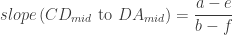, making those two midpoint segments parallel.  Likewise, , proving the other opposite side pair also was parallel.  With both pairs of opposite sides parallel, the midpoint quadrilateral was necessarily a parallelogram.

I had two groups leverage the fact that the diagonals of parallelograms were mutually bisecting.     .  QED.

One student even proved that opposite sides were congruent.

While it was not readily available for my students this year, I can imagine allowing CAS for these manipulations if I use this activity in the future.

EXTENDING THE QMT TO SIMILARITY:  For the next stage, I asked my students to explains what happens when the QMT is applied to degenerate quadrilaterals.

PART II:  You could think of triangles as being degenerate quadrilaterals when two quadrilateral vertices coincide to make one side of the quadrilateral have side length 0.  Apply this to generic quadrilateral ABCD from above where points A and D coincide to create triangle BCD.  Use this to explain how the segment connecting the midpoints of any two sides of a triangle is related to the third side of the triangle.

I encourage you to construct this using a dynamic geometry package, but here’s the result.

 

Heres a brief video showing the quadrilateral going degenerate.

Notice the parallelogram still exists and forms two midpoint segments on the triangle (degenerate quadrilateral).  By parallelogram properties, each of these segments is parallel and congruent to the opposite side of the parallelogram, making them parallel to and half the length of the opposite side of the triangle.

CONCLUSION:  I think it critical to teach in a way that draws connections between ideas and units. This exercise made a lovely transition from quadrilaterals through coordinate proofs to the triangle midpoint theorem.