Best Algebra 2 Lab Ever

This post shares what I think is one of the best, inclusive, data-oriented labs for a second year algebra class.  This single experiment produces linear, quadratic, and exponential (and logarithmic) data from a lab my Algebra 2 students completed this past summer.  In that class, I assigned frequent labs where students gathered real data, determined models to fit that data, and analyzed goodness of the models’ fit to the data.   I believe in the importance of doing so much more than just writing an equation and moving on.

For kicks, I’ll derive an approximation for the coefficient of gravity at the end.

THE LAB:

On the way to school one morning last summer, I grabbed one of my daughters’ “almost fully inflated” kickballs and attached a TI CBR2 to my laptop and gathered (distance, time) data from bouncing the ball under the Motion Sensor.  NOTE:  TI’s CBR2 can connect directly to their Nspire and TI84 families of graphing calculators.  I typically use computer-based Nspire CAS software, so I connected the CBR via my laptop’s USB port.  It’s crazy easy to use.

One student held the CBR2 about 1.5-2 meters above the ground while another held the ball steady about 20 cm below the CBR2 sensor.  When the second student released the ball, a third clicked a button on my laptop to gather the data:  time every 0.05 seconds and height from the ground.  The graphed data is shown below.  In case you don’t have access to a CBR or other data gathering devices, I’ve uploaded my students’ data in this Excel file.

Remember, this is data was collected under far-from-ideal conditions.  I picked up a kickball my kids left outside on my way to class.  The sensor was handheld and likely wobbled some, and the ball was dropped on the well-worn carpet of our classroom floor.  It is also likely the ball did not remain perfectly under the sensor the entire time.  Even so, my students created a very pretty graph on their first try.

For further context, we did this lab in the middle of our quadratics unit that was preceded by a unit on linear functions and another on exponential and logarithmic functions.  So what can we learn from the bouncing ball data?

LINEAR 1:  

While it is very unlikely that any of the recorded data points were precisely at maximums, they are close enough to create a nice linear pattern.

As the height of a ball above the ground helps determine the height of its next bounce (height before –> energy on impact –> height after), the eight ordered pairs (max height #n, max height #(n+1) ) from my students’ data are shown below

This looks very linear.  Fitting a linear regression and analyzing the residuals gives the following.

The data seems to be close to the line, and the residuals are relatively small, about evenly distributed above and below the line, and there is no apparent pattern to their distribution.  This confirms that the regression equation, , is a good fit for the x = height before bounce and y = height after bounce data.

NOTE:  You could reasonably easily gather this data sans any technology.  Have teams of students release a ball from different measured heights while others carefully identify the rebound heights.

The coefficients also have meaning.  The 0.673 suggests that after each bounce, the ball rebounded to 67.3%, or 2/3, of its previous height–not bad for a ball plucked from a driveway that morning.  Also, the y-intercept, 0.000233, is essentially zero, suggesting that a ball released 0 meters from the ground would rebound to basically 0 meters above the ground.  That this isn’t exactly zero is a small measure of error in the experiment.

EXPONENTIAL:

Using the same idea, consider data of the form (x,y) = (bounce number, bounce height). the graph of the nine points from my students’ data is:

This could be power or exponential data–something you should confirm for yourself–but an exponential regression and its residuals show

While something of a pattern seems to exist, the other residual criteria are met, making the exponential regression a reasonably good model: .  That means bounce number 0, the initial release height from which the downward movement on the far left of the initial scatterplot can be seen, is 0.972 meters, and the constant multiplier is about 0.676.  This second number represents the percentage of height maintained from each previous bounce, and is therefore the percentage rebound.  Also note that this is essentially the same value as the slope from the previous linear example, confirming that the ball we used basically maintained slightly more than 2/3 of its height from one bounce to the next.

And you can get logarithms from these data if you use the equation to determine, for example, which bounces exceed 0.2 meters.

So, bounces 1-4 satisfy the requirement for exceeding 0.20 meters, as confirmed by the data.

A second way to invoke logarithms is to reverse the data.  Graphing x=height and y=bounce number will also produce the desired effect.

QUADRATIC:

Each individual bounce looks like an inverted parabola.  If you remember a little physics, the moment after the ball leaves the ground after each bounce, it is essentially in free-fall, a situation defined by quadratic movement if you ignore air resistance–something we can safely assume given the very short duration of each bounce.

I had eight complete bounces I could use, but chose the first to have as many data points as possible to model.  As it was impossible to know whether the lowest point on each end of any data set came from the ball moving up or down, I omitted the first and last point in each set.  Using (x,y) = (time, height of first bounce) data, my students got:

What a pretty parabola.  Fitting a quadratic regression (or manually fitting one, if that’s more appropriate for your classes), I get:

Again, there’s maybe a slight pattern, but all but two points are will withing  0.1 of 1% of the model and are 1/2 above and 1/2 below.  The model, , could be interpreted in terms of the physics formula for an object in free fall, but I’ll postpone that for a moment.

LINEAR 2:

If your second year algebra class has explored common differences, your students could explore second common differences to confirm the quadratic nature of the data.  Other than the first two differences (far right column below), the second common difference of all data points is roughly 0.024.  This raises suspicions that my student’s hand holding the CBR2 may have wiggled during the data collection.

Since the second common differences are roughly constant, the original data must have been quadratic, and the first common differences linear. As a small variation for each consecutive pair of (time, height) points, I had my students graph (x,y) = (x midpoint, slope between two points):

If you get the common difference discussion, the linearity of this graph is not surprising.  Despite those conversations, most of my students seem completely surprised by this pattern emerging from the quadratic data.  I guess they didn’t really “get” what common differences–or the closely related slope–meant until this point.

Other than the first three points, the model seems very strong.  The coefficients tell an even more interesting story.

GRAVITY:

The equation from the last linear regression is .  Since the data came from slope, the y-intercept, 4.55, is measured in m/sec.  That makes it the velocity of the ball at the moment (t=0) the ball left the ground.  Nice.

The slope of this line is -9.61.  As this is a slope, its units are the y-units over the x-units, or (m/sec)/(sec).  That is, meters per squared second.  And those are the units for gravity!  That means my students measured, hidden within their data, an approximation for coefficient of gravity by bouncing an outdoor ball on a well-worn carpet with a mildly wobbly hand holding a CBR2.  The gravitational constant at sea-level on Earth is about -9.807 m/sec^2.  That means, my students measurement error was about 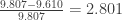.  And 2.8% is not a bad measurement for a very unscientific setting!

CONCLUSION:

Whenever I teach second year algebra classes, I find it extremely valuable to have students gather real data whenever possible and with every new function, determine models to fit their data, and analyze the goodness of the model’s fit to the data.  In addition to these activities just being good mathematics explorations, I believe they do an excellent job exposing students to a few topics often underrepresented in many secondary math classes:  numerical representations and methods, experimentation, and introduction to statistics.  Hopefully some of the ideas shared here will inspire you to help your students experience more.

Exploring Sequences and Lines

Here’s another favorite problem that could be used for any middle or high school students who’ve been exposed to both arithmetic sequences and linear equations.

There is a family of lines, , for which can be any arithmetic sequence.  What do all members of this family have in common?

As with most great math problems, the problem is simply stated and can be approached from many different perspectives.  In the end, this one isn’t that difficult to crack, but the solution (at least to me) is not intuitively obvious from the problem statement. If you’ve not seen this before, please try it before reading further.

WARNING:  Problem Solution Follows

MOST COMMON STUDENT APPROACH:  Given the problem’s phrasing, most begin by writing out a few possible equations using different arithmetic sequences, typically with positive common differences.  After a few tries, most get a little frustrated as no obvious pattern emerges from the equations.

It is this point that is typically the most difficult for me as a teacher.  I want to help anyone who struggles, but “help” often means allowing others the room to struggle and to find ways of solving problems on their own.  Only when a student or group gets really frustrated do I sometimes ask, “Are there any other ways you can look at this problem or at your work?”

Eventually, most decide to graph their equations to see if anything pops out.  The following graph was submitted this past semester by one of my precalculus students using the free online Desmos calculator.

Two lines intersecting in a point is common.  Three or more in a single point almost always indicates something interesting.  Seven lines through a single point is screaming for attention!  From this graph, all lines in this family apparently contain the point (1,-2).  That seems a bit random until you investigate further, but pattern recognition is just half of the battle for a mathematician.  Now that something interesting has been discovered, a mathematician wants to know if this is a fluke or something inherent to all members of the family.

NOTE:  All graphs my students have produced over the years have always contained specific equations.  I don’t know that it’s any more enlightening, but I did create on Desmos a slider version of the graphs of this family with one slider for the initial term (A) and a second for its common difference (d).

UNIQUE SOLUTION METHODS FROM STUDENTS:

All successful solutions eventually rewrite the sequence to where d is the common difference for a generic arithmetic sequence with initial term A.

Method I: After discovering the common point of intersection, most plug it into the left side of the equation and simplify to get

.

Because the left side reduces to zero for all generic arithmetic sequences, , (1,-2) must be common to all members of this family.

A few students aren’t comfortable dealing with 0=0, so these tend to plug in and solve for y to get , proving that the y-coordinate for for all members of this family is always -2.

Method II:  A few students every year work algebraically from properties of arithmetic sequences.  For any arithmetic sequence, , .  This rewrites to , so whenever , then  is a fundamental property of all arithmetic sequences.

Personally, I think this method gets closest to explaining why the point (1,-2) is the common characteristic of this family.

Method III:  This year, I had a student take an approach I’d never seen before.  She defined one arithmetic sequence as and another as  for any real values of a,d,m, and n.  This leads to a system of equations:  and  .  If you have some younger students or if all the variables make you nervous, the solution is available via Wolfram Alpha.

Still, this system is pretty easy to manipulate.  If you multiply the first equation by m and the second by a, the x-terms will eliminate with subtraction, giving

.

Solving for y shows that all of the coefficients simplify surprisingly easily.

From here, determining is easy, proving the relationship.

SOLUTIONS and APPROACHES NOT YET OFFERED BY STUDENTS:

Approach A:  High school students don’t often think about ways to simplify problem situations, especially at the beginning of problems.  One way I did that for this problem in later class discussions was to recognize that it one of the terms in the arithmetic sequence was 0, you didn’t need to deal with nearly as many terms. For example, if your sequence was , the linear equation would be .  Similarly, the sequence leads to .  Obviously, the only thing these two lines have in common is the point (1,-2).  A proof of the property must still be established, but this is one of the fastest ways I’ve seen to identify the central property.

Approach B:  A purely algebraic approach to this problem could redefine the arithmetic sequence as as before, giving:

Collecting like terms gives

.

The values of a and d must remain as parameters to include all possible arithmetic sequences.  Because the equation always equals 0, the coefficients of a and d are both 0, making (for the coefficient of d) and therefore .

EXTENSION:

We once had a test question at the end of the unit containing this exercise.  Basically, it reminded students that they had discovered that all lines , for which can be any arithmetic sequence contained the point (1,-2).  It then asked for an equation of a family of linear functions using the same arithmetic  that all contained the point (1,2).

The two most common responses we’ve seen involve a reflection or a vertical translation.  (1,-2) can become (1,2) by reflecting over the x-axis, so making the y-values negative would do the trick:  .  Similarly, (1,-2) can become (1,2) by translating up 4 units, giving .

In Plain Sight, but Unseen

Thanks to a comment from Doug Kuhlmann on my last post, I’ve got a few new cool connections on the transformational effects of the parameters in on its graph.  This is exactly why I share.  Thanks, Doug!!

THE NEW PATTERN:  Use this GeoGebraTube Web document to model the problem.  Set the value of b to any non-zero value and vary a.  The parabola’s vertex moves along a line, as shown below.

As with the changes in the b parameter, define that line and prove your claims.

[The GeoGebra link above does not produce the vertex geometry trace footprints shown in the image.  If you want to create these, download GeoGebra and create this simple document for yourself.  It is FREE.  If anyone wants explicit instructions for how to do this, email me and I’ll post instructions on the ‘blog.]

Another option to see the line is to use Geogebra’s locus tool.  It requires two inputs:  which object is the locus following, and which variable driving the variation.  After selecting the locus tool, click on the vertex and then the slider for a.  You get the next image.

SOLUTION ALERT!  Don’t read further if you want to solve the problem for yourself.

I knew the line contained the vertex and noticed that it seemed to pass through y-intercept.  Predicting the y-intercept was c, all I needed was the slope.  With my prediction of the two generic points, I could compute that, too.  I enjoy symbol manipulation for the mental exercise.  The symbols (to me) weren’t all that complicated, so I took a brief moment of fun solving that by hand.  But this is another of those situations where the symbol manipulation isn’t the point, so using my CAS is 100% legitimate.  It is also a great leveler of ability for those intimidated for any reason by algebraic manipulations.

The next image is a great use of CAS commands to find the line’s slope.  In particular, notice the use of a function definition to minimize the algebraic clutter through function notation.

Lovely and surprisingly simple.  That means the line the parabola’s vertex follows when a varies for non-zero b is .

Students often overlook the domain warning.  It doesn’t matter for the creation of the line, but ultimately lies at the heart of the unequal spacing of the vertex footprints in the first image and explains the unique behavior of the parabola’s movement.

If a student didn’t use the vertex and y-intercept to derive the linear equation, a CAS solve command could legitimately be used to show that those two generic points were always on the line.

MOTION ALONG THE LINE:  One of the interesting parts of this problem is how the parabola moves along .  After some play with the GeoGebra document, you can see that as the parabolas’ vertices move infinitely far away from the y-axis, and as  the vertices approach the y-axis. This also can be seen numerically from the generic x-coordinate of the vertex, .  For a fixed, non-zero value of b, the fraction representing the x-coordinate of the vertex increases in magnitude as and decreases in magnitude toward 0 as .

The vertex trace points in the first image above are separated by .  The reason for the differences in distances between the points noted above is because does not change linearly when a changes linearly.  As , slower and slower, explaining the increasing density of the vertex trace points near the y-axis.

When , the x-coordinate of the vertex is undefined.  At that moment, the generic quadratic, , becomes the degenerate , a line.  Graphing that line (the red dashed line below) against a trace of all possible parabolas as a varies, the degenerate parabola resulting when is precisely the tangent line to all of these parabolas at their y-intercept, –a pretty extension on a connection suggested by Dave Radcliffe on a cross-posting of my initial post.  Nice.

A FINAL NOTE:  My memory suggests that I’ve seen this pattern before in some of the numerous times I’ve presented the b-variation of this problem in conferences and assigned it in classes.  Despite all the times I must have seen it, the pattern never rose to my active conscience.  Serendipitously, I’m currently reading Tina Seelig’s inGenius:  A Crash Course on Creativity. I offer two quotes from her Are You Paying Attention? chapter:

• We think we understand the world and look for the patterns that we already recognize. (p. 71)
• We focus predominantly on things that are at our eye level rather than looking around more broadly.  In addition, we pay attention to objects that we expect to find and ignore those things that don’t fit. (p. 71)

The moral:  Even after all of my attempts and success at finding unique patterns, I missed this one until Doug pointed it out to me.  I suspect my focus on what I knew about b‘s effect blinded me to the a effect.  This is a great reminder to me to always hold myself ready to see beauty and pattern in unexpected places.