Inscribed Triangle Challenge

@MathCeyhun posed an interesting geometry problem yesterday.

Area(ABC)=? pic.twitter.com/pRBmetivx7

— Ceyhun Köylüce (@MathCeyhun) September 21, 2018

Even more interesting is that, as @MathCeyhun noted in a subsequent tweet, none of the posted solutions is correct.  There have been a few posted answers, but no solutions, so I thought I’d give it a try.

OBSERVATIONS

• The perpendicular bisector of each chord was given, and perpendicular bisectors of chords always lie on radii of the circle.
• If r is the radius of the circle, then the lengths of the extensions of the perpendicular bisectors are r-1, r-2, and r-3.
• Nothing given guarantees anything special about the triangle, so I assumed it was scalene.  I called the side lengths 2x, 2y, and 2z to simplify the bisection labels.
• Adding the bisector extensions, the radii to the vertices, and segment names and labels gave me this.

[Irrelevant to this problem, but I just realized by looking at this image that every triangle can be dissected into three isosceles triangles with congruent sides and a shared vertex point at the triangle’s circumcenter.  Pretty.]

SETTING UP MY SOLUTION 

Each isosceles triangle is bisected by the perpendicular bisector of its base from which I extracted three relationships from the Pythagorean theorem.

[The relationship between the half-sides, the extension of the radius beyond the triangle, and the radius is another pretty pattern.]

That gives 3 equations in 4 variables.  I needed one more to solve….

 

The area of can be expressed two ways:  as the sum of the areas of the isosceles triangles, and using Heron’s formula.  From the areas of the isosceles triangles,

The sides of are 2x, 2y, and 2z, so its semiperimeter is x+y+z and Heron’s formula gives its area as

.

The area of a given triangle is unique, so the two different area expressions are equivalent, giving a fourth equation.

SOLVING A SYSTEM & ANSWERING THE QUESTION

With four equations in four variables, I had a system of equations.  The algebra was messy, so I invoked my CAS to crunch it for me.

The question asked for the area of the triangle, so I just substituted my values back into the area formulas.

And 17.186… is clearly not one of the choices in the original problem.

 

A PLEA…

Recognizing the perpendicular bisectors, seeing all the right triangles, and connecting the multiple ways to describe the area of a triangle made this solution reasonably easy to find with the help of my computer algebra system (CAS), but I know the background algebra is, at best, cumbersome.  I hope there’s a more elegant solution, but I don’t see it.  Can anyone offer a suggestion?

Either way … this is definitely becoming a challenge problem for my Quantitative Reasoning class this coming week!

Implicit Derivative Question

Yesterday, this question posted within the AP Calculus Community about implicit derivatives.

Below, I argue why the derivatives MUST be the same, show how four different variations can all be shown to give the same derivative, and provide a final conclusion.

INITIAL INTUITION

The Desmos graph of the given relation, is , is shown below.  Logically, it seems that even when the terms of the relation are algebraically rearranged, the graph should be invariant.   The other two forms mentioned in the Community post are on lines 2 and 3.  Lines 4, 5, and 6 show three other variations.  Here is the link to my Desmos graph allowing you to change between the forms to visually confirm the graphical invariance intuition.

If calculus “works”, it also shouldn’t matter how one calculates a derivative.   While the forms of the derivative certainly could LOOK different,  because any point on the invariant graph has the same tangent line no matter what the form of its equation, and the derivative of a relation at a point is the slope of that invariant tangent line, then the derivative also MUST be invariant.

CALCULATING “DIFFERENT” DERIVATIVES

To show the derivatives are fundamentally all the same (as suspected by the initial post), I calculate the derivatives of the equations on lines 1 and 3 given in the initial post as well as my variations on lines 4 and 6.

LINE 1:

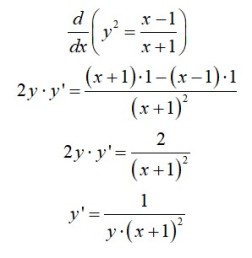
Using the Chain Rule on the left and the Quotient Rule on the right gives

LINE 3:

This version is more complicated, requiring the Product Rule in addition to the earlier Chain and Quotient Rules.  In the penultimate line, I used the original equation to substitute for to transform the derivative into the same form as line 1.

LINE 4:

This time, differentiation requires only the Chain and Product Rules.

After the usual substitution for , I multiplied both sides by to clear the denominator and solved for , returning the same result.

LINE 6:

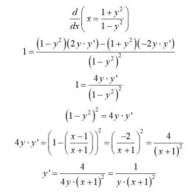
This time, the relation is solved for x, resulting in a much more complicated Quotient+Chain Rule calculation, but substituting for and changing the form leads once again to the same answer.

Hopefully this is convincing evidence that all derivative forms can be shown to be equivalent.   If you’re still learning implicit differentiation, I encourage you to show the derivatives from the lines 2 and 5 variations are also equivalent.

CONCLUSION

So which approach is “best”?  In my opinion, it all depends on your personal comfort with algebraic manipulations.  Some prefer to just take a derivative from the given form of .  I avoid the more complicated quotient rule whenever I can, so the variation from line 4 would have been my approach.

The cool part is that it doesn’t matter what approach you use, so long as your algebraic manipulations are sound.  You don’t have to accept the form in which a problem is given; CHANGE IT to a form that works for you!

Pythagorean Investigation

 

Here’s a challenge @jamestanton tweeted yesterday:

Can the hypotenuse and one side length of one right integer triangle be the two side lengths of another right integer triangle?

— James Tanton (@jamestanton) September 9, 2018

Visually, Tanton is asking if there is an integer right triangle (like the standard version shown on the left below) for which the integer triangle on the right exists.

The algebraic equivalent to this question is, for some , does there exist a Natural number d so that ?

I invoked Euclid’s formula in my investigation to show that there is no value of d to make this possible.  I’d love to hear of any other proof variations.

INVOKING EUCLID’S FORMULA

For any coprime natural numbers m & n where and is odd, then every primitive Pythagorean triple can be generated by .

For any Natural number k, every Pythagorean triple can be generated by .

The generator term must be the original hypotenuse (side c), but either or can be side b.  So, if Tanton’s scenario is true, I needed to check two possible cases.  Does there exist a Natural number d such that

or

is true?

EVALUATING THE POSSIBILITIES

For the first equation, there is a single factor of 2 on the right, and there is no way to extract an odd number of factors of 2 from or , so can’t represent a perfect square.

For the second equation, there is no way to factor over Integers, so can’t be a perfect square either.

Since neither equation can create a perfect square, there is no Natural value of d that makes {b, c, d} a Pythagorean triple.  Tanton’s challenge is impossible.

Does anyone have a different approach?

Deep Unit Circle Understanding

Chris Bolognese started a new Honors Trigonometry unit a few days ago and posted a new problem set, welcoming feedback.  Clicking on the document image gives you access to Chris’ problem set.

https://twitter.com/EulersNephew/status/1033118502171881473

This post is my feedback.  I wrote it as a conversation with Chris.  it

 

FEEDBACK…

Question 2 suggests you have already discussed special angles (or your students recalled them from last year’s algebra class).  What I love about this problem set is how you shift the early focus away from these memorized special angles and onto the deep symmetry underlying the unit circle (and all of trigonometry).  Understanding deep structure grants always far more understanding than rote memorizations ever does!

HINTS OF IDENTITIES TO COME…

The problem set’s initial exploration of trig symmetry starts in parts a-d of Question 1, asking students to justify statements like and .  The symmetry is nice, and I hope you refer back to this problem set when your class turns to its formal exploration of trig identities, helping them see that not all proofs of identities require algebraic justifications.

CONSIDERATION 1:  Put some creative power in your students’ hands.  Challenge them to discover additional algebraic/transformational identities like Questions 1a-1d.  For example, what is the relationship between and  ?  There are LOTS of symmetry statements they could write.

CONSIDERATION 2:  I would shift Question 1e to Question 4, as 1e is the basis of the Pythagorean identities you explore in the later group.

CONSIDERATION 3:  I suggest dropping Question 4d and asking students to discover another equation showing another Pythagorean relationship between trig functions.  That cotangent and cosecant have not yet been used is hopefully a loud, silent hint.

CONSIDERATION 4:  They’re not ready for this one until they see sinusoidal graphs, but another trig pre-identity I love is graphing and asking students to write an equivalent equation using only translations and dilations.

Unlike the symmetric relationships in 1a-1d, I don’t think you can actually KNOW it is true without algebraic relationships.  I use problems like this to set up and justify the transition to identities.

 

VERY CLEVER SUMMATIONS …

I don’t recall ever seeing something like your Question 3 before.  In my opinion, is the gold nugget in the assignment, especially with your students’ prior exposure to special angles.

CONSIDERATION 5:  In some ways the large number of addends in  gives away that there must be a simpler approach than the problem suggests on its surface.  What about something that suggests a direct solution if you don’t invoke the symmetry, like ?

CONSIDERATION 6:  Closely related to this, why not shamelessly take advantage of the memorized values to see if students notice the symmetry to notice a simpler approach?  I suggest , with sine or cosine.

CONSIDERATION 7:  My prior two examples tweaked your initial  problem.  Like Consideration 1, why not challenge your students to develop their own summations?  I bet they can develop some clever alternatives.

 

DO YOU UNDERSTAND RADIANS???

In Question 3, you had some nice explorations using degrees.  Unfortunately, I’m not aware of many equally clever early questions involving radians that aren’t degree-oriented in disguise.  Here are my final suggestions to address this gap.

CONSIDERATION 8:  Without using any technology, rank

sin(1), cos(2), tan(3), cot(4), sec(5), csc(6)

in ascending order.  Note that all angles are expressed in radian measures.  One pair of expressions is very difficult.  (A softer version of this question ranks only sin(1), cos(2), & tan(3).)

CONSIDERATION 9:  One pair of expressions in Consideration 8 is very difficult to rank without technology.  Which pair is this and why is it so difficult to rank?  Exchange angles or functions to change this question in a way that makes it easier to rank.

 

Thanks for the fun and thoughtful problem set.

FiveThirtyEight Riddler Express Solution

I’d not peeked at FiveThirtyEight’s The Riddler in a while when I saw Neema Salimi ‘s post about the June 22, 2018 Riddler Express   Neema argued his solution was accessible to Algebra 1 students–not always possible for FiveThirtyEight’s great logic puzzles–so I knew it was past time to return.

After my exploration, I’ve concluded this is DEFINITELY worth posing to any middle school learners (or others) in search of an interesting problem variation.

Following is my solution, three retrospective insights about the problem, a comparison to Neema’s solution, and a proposed alternative numeric approach I think many Algebra 1 students might actually attempt.

THE PROBLEM:

Here is a screenshot of the original problem posted on FiveThirtyEight (2nd item on this page).

If you’re familiar with rate problems from Algebra 1, this should strike you immediately as a “complexification” of type problems.  (“Complexification” is what a former student from a couple years ago said happened to otherwise simple problems when I made them “more interesting.”)

MY SOLUTION:

My first thought simplified my later algebra and made for a much more dramatic ending!!  Since Michelle caught up with her boarding pass with 10 meters left on the walkway, I recognized those extra 10 meters as irrelevant, so I changed the initial problem to an equivalent question–from an initial 100 m to 90 m–having Michelle catch up with her boarding pass just as the belt was about to roll back under the floor!

Let W = the speed of the walkway in m/s.  Because Michelle’s boarding pass then traveled a distance of 90 m in W m/s, her boarding pass traveled a total seconds.

If M = Michelle’s walking speed, then her total distance traveled is the initial 90 meters PLUS the distance she traveled in the additional 90 seconds after dropping her boarding pass.  Her speed at this time was   m/s (subtracting W because she was moving against the walkway), so the additional distance she traveled was , making her her total distance .

Then Michelle realized she had dropped her boarding pass and turned to run back at m/s (adding to show moving with the walkway this time), and she had seconds to catch it before it disappeared beneath the belt.  The subtraction is the time difference between losing the pass and realizing she lost it.  Substituting into  gives

A little expansion and algebra cleanup …

And multiplying by solves the problem:

INSIGHTS:

Insight #1:  Solving a problem is always nice, but I was thinking all along that I pulled off my solution because I’m very comfortable with algebraic notation.  This is certainly NOT true of most Algebra 1 students.

Insight #2:  This made me wonder about the viability of a numeric solution to the problem–an approach many first-year algebra students attempt when frutstrated.

Insight #3:  In the very last solution step, Michelle’s rate, M, completely dropped out of the problem.  That means the solution to this problem is independent of Michelle’s walking speed.

Wondering if other terms might be superfluous, too, I generalized my initial algebraic solution further with A = the initial distance before Michelle dropped her boarding pass and B = the additional time Michelle walked before realizing she had dropped the pass.

And solving for W gives .

So, the solution does depend on the initial distance traveled and the time before Michelle turns around, and it was simplified in the initial statement with .  That all made sense after a few quick thought experiments.  With one more variation you can show that the scale factor between her walking and jogging speed is relevant, but not her walking speed.  But now it was clear that in all cases, Michelle’s walking speed is irrelevant!

COMPARING TO NEEMA:

My initial conclusion matched Neema’s solution, but I really liked my separate discovery that the answer was completely independent of Michelle’s walking speed.  In my opinion, those cool insights are not at all intuitive.

AN ALTERNATIVE NUMERIC APPROACH:

While this approach is just a series of special cases of the generic approach, I suspect many Algebra 1 students would likely get frustrated quickly by the multiple variable and attempt

Ignoring everything above, but using the same variables for simplicity, perhaps the easiest start is to assume the walkway moves at W=1 m/s and Michelle’s walking speed is M=2 m/s.  That means her outward speed against the walkway is (2-1) = 1 m/s.  She drops the pass at 90 meters after 90 seconds.  So the pass will be back at the start after 90 seconds, the additional time that Michelle walks before realizing her loss.

I could imagine many students I’ve taught working from this through some sort of intelligent numeric guess-and-check, adjusting the values of M and W until landing at .  The fractional value of W would slow them down, but many would get it this way.

CONCLUSION:

I’m definitely pitching this question to my students in just a few weeks.  (Where did summer go?)  I’m deeply curious about how they’ll approach their solutions.  I”m convinced many will attempt–at least initially–playing with more comprehensible numbers.  Such approaches often give young learners the insights they need to handle algebra’s generalizations.

Painting and Probability

 

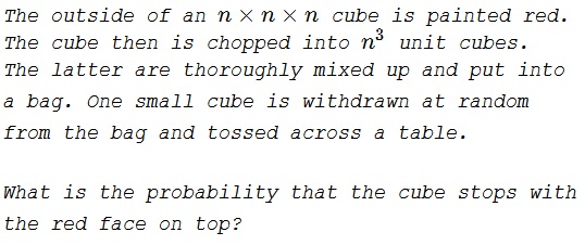
Here’s a cool probability problem the start of which is accessible to middle and high school students with careful reasoning.  It was posted by Alexander Bogomolny on Cut the Knot a week ago. I offer what I think is a cool extension of the problem following the initial credits.

The next day Mike Lawler tweeted another phenomenal video solution worked out with his boys during Family Math.

What kids learning math can look like -> Working through a terrific probability problem shared by Alexander Bogomolny yesterday: https://t.co/NR7j7Zh6hS #math #mathchat cc: @CutTheKnotMath

— Mike Lawler (@mikeandallie) March 25, 2018

Mike’s videos show his boys thinking through simpler discrete cases of the problem and their eventual case-by-case solution to the nxnxn question.  The last video on the page gives a lovely alternative solution completely bypassing the case-by-case analyses.  This is also “Solution 1” on Alexander’s page.

EXTENDING THE PROBLEM:

When I first encountered the problem, I wanted to think about it before reading any solutions.  As with Mike’s boys, I was surprised early on when the probability for a 2x2x2 cube was and the probability for a 3x3x3 cube was .  That was far too pretty to be a coincidence.  My solution exactly mirrored the nxnxn case-by-case analysis in Mike’s videos:  the probability of rolling a painted red face up from a randomly selected smaller cube is .

Surely something this simple and clean could be generalized.  Since a cube can be considered a “3-dimensional square”, I re-phrased Alexander’s question into two dimensions.  The trickier part was thinking what it would mean to “roll” a 2-dimensional shape.

The outside of an nxn square is painted red and is chopped into unit squares.  The latter are thoroughly mixed up and put into a bag.  One small square is withdrawn at random from the bag and spun on a flat surface.  What is the probability that the spinner stops with a red side facing you?

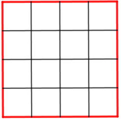
Shown below is a 4×4 square, but in all sizes of 2-dimensional squares, there are three possible types in the bag:  those with 2, 1, or 0 sides painted.

I solved my first variation case by case.  In any nxn square,

• There are 4 corner squares with 2 sides painted.  The probability of picking one of those squares and then spinning a red side is .
• There are edge squares not in a corner with 1 side painted.  The probability of picking one of those squares and then spinning a red side is .
• All other squares have 0 sides painted, so the probability of picking one of those squares and then spinning a red side is 0.
• Adding the probabilities for the separate cases gives the total probability: 

After reading Mike’s and Alexander’s posts, I saw a much easier approach.

• Paint all 4 edges of an nxn square, and divide each painted edge into n painted unit segments.  This creates total painted small segments.
• Decompose the nxn original square into unit squares.  Each unit square has 4 edges giving total edges.
• Because every edge of every unit square is equally likely to be spun, the total probability of randomly selecting a smaller square and spinning a red side is .

The dimensions of the “square” don’t seem to matter!

WARNING: 

Oliver Wendell Holmes noted, “A mind that is stretched by a new experience can never go back to its old dimensions.”  The math after this point has the potential to stretch…

EXTENDING THE PROBLEM MORE:

I now wondered whether this was a general property.

In the 2-dimensional square, 1-dimensional edges were painted and the square was spun to find the probability of a red edge facing.  With the originally posed cube, 2-dimensional faces were painted and the cube was tossed to find the probability of an upward-facing red face.  These cases suggest that when a cube of some dimension with edge length n is painted, is decomposed into unit cubes of the original dimension, and is spun/tossed to show a cube of one smaller dimension, then the probability of getting a painted smaller-dimensional cube of is always , independent of the dimensions occupied by the cube.

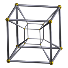
Going beyond the experiences of typical middle or high school students, I calculated this probability for a 4-dimensional hypercube (a tesseract).

• The exterior of a tesseract is 8 cubes.  Ignore the philosophical difficulty of what it means to “paint” (perhaps fill?) an entire cube.  After all, we’re already beyond the experience of our 3-dimensions.
• Paint/fill all 8 cubes on the surface of the tesseract, and divide each painted cube into painted unit cubes.  This creates total painted unit cubes.
• Decompose the original tesseract into unit tesseracts.  Each unit tesseract has 8 cubes giving total unit cubes.
• Because every unit cube on every unit tesseract is equally likely to be “rolled”, the total probability of randomly selecting a smaller tesseract and rolling a red cube is .

The probability is independent of dimension! 

More formally,

The exterior of a d-dimensional hypercube with edge length n is painted red and is chopped into unit d-dimensional hypercubes.  The latter are put into a bag of sufficient dimension to hold them and thoroughly mixed up.  A unit d-dimensional hypercube is withdrawn at random from the bag and tossed.  The probability that the unit d-dimensional hypercube lands with a red (d-1)-dimensional hypercube showing is .

PROOF:

• The exterior of a d-dimensional hypercube is comprised of 2d (d-1)-dimensional hypercubes of dimension (d-1).  Paint/fill all 2d surface hypercubes and divide each painted (d-1)-dimensional hypercube into painted unit hypercubes.  This creates total painted unit hypercubes.
• Decompose the original tesseract into unit d-dimensional hypercubes.  Each unit d-dimensional hypercube has 2d surface (d-1)-dimensional hypercubes giving total surface unit d-dimensional hypercubes.
• Because every unit (d-1)-dimensional hypercube on the surface of every unit d-dimensional hypercube is equally likely to be “rolled”, the total probability of randomly selecting a unit d-dimensional hypercube and rolling a (d-1)-dimensional red-painted hypercube is .

 

I hope you can now return to something close to your old dimensions.

Inscribed Right Angle Proof Without Words

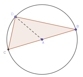
Earlier this past week, I assigned the following problem to my 8th grade Geometry class for homework.  They had not explored the relationships between circles and inscribed angles, so I added dashed auxiliary segment AD as a hint.

What follows first is the algebraic solution I expected most to find and then an elegant transformational explanation one of my students produced.

PROOF 1:

Given circle A with diameter BC and point D on the circle.  Prove triangle BCD is a right triangle.

After some initial explorations on GeoGebra sliding point D around to discover that its angle measure was always independent of the location of D, most successful solutions recognized congruent radii AB, AC, and AD, creating isosceles triangles CAD and BAD.  That gave congruent base angles x in triangle CAD, and y in BAD.

The interior angle sum of a triangle gave , or , confirming that BCD was a right triangle.

PROOF 2:

Then, one student surprised us.  She marked the isosceles base angles as above before rotating about point A.

Because the diameter rotated onto itself, the image and pre-image combined to form an quadrilateral with all angles congruent.  Because every equiangular quadrilateral is a rectangle, M had confirmed BCD was a right triangle.

CONCLUSION:

I don’t recall seeing M’s proof before, but I found it a delightfully elegant application of quadrilateral properties.  In my opinion, her rotation is a beautiful proof without words solution.

Encourage freedom, flexibility of thought, and creativity, and be prepared to be surprised by your students’ discoveries!

Quadratics + Tangent = ???

 

Here’s a very pretty problem I encountered on Twitter from Mike Lawler 1.5 months ago.

Really interesting and clever challenge problem in my son's trig book: Find the sum of the solutions between 0 and 2 PI of the equation (Tan(x))^2 – 9*Tan(x) + 1 = 0.

— Mike Lawler (@mikeandallie) November 23, 2017

I’m late to the game replying to Mike’s post, but this problem is the most lovely combination of features of quadratic and trigonometric functions I’ve ever encountered in a single question, so I couldn’t resist.  This one is well worth the time for you to explore on your own before reading further.

My full thoughts and explorations follow.  I have landed on some nice insights and what I believe is an elegant solution (in Insight #5 below).  Leading up to that, I share the chronology of my investigations and thought processes.  As always, all feedback is welcome.

WARNING:  HINTS AND SOLUTIONS FOLLOW

Investigation  #1:

My first thoughts were influenced by spoilers posted as quick replies to Mike’s post.  The coefficients of the underlying quadratic, , say that the solutions to the quadratic sum to 9 and multiply to 1.  The product of 1 turned out to be critical, but I didn’t see just how central it was until I had explored further.  I didn’t immediately recognize the 9 as a red herring.

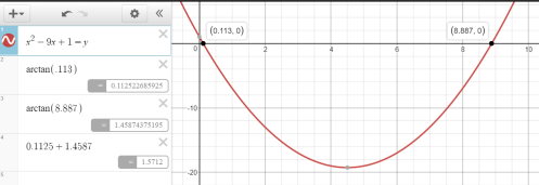
Basic trig experience (and a response spoiler) suggested the angle values for the tangent embedded in the quadratic weren’t common angles, so I jumped to Desmos first.  I knew the graph of the overall given equation would be ugly, so I initially solved the equation by graphing the quadratic, computing arctangents, and adding.

Insight #1:  A Curious Sum

The sum of the arctangent solutions was about 1.57…, a decimal form suspiciously suggesting a sum of .  I wasn’t yet worried about all solutions in the required interval, but for whatever strange angles were determined by this equation, their sum was strangely pretty and succinct.  If this worked for a seemingly random sum of 9 for the tangent solutions, perhaps it would work for others.

Unfortunately, Desmos is not a CAS, so I turned to GeoGebra for more power.

Investigation #2:  

In GeoGebra, I created a sketch to vary the linear coefficient of the quadratic and to dynamically calculate angle sums.  My procedure is noted at the end of this post.  You can play with my GeoGebra sketch here.

The x-coordinate of point G is the sum of the angles of the first two solutions of the tangent solutions.

Likewise, the x-coordinate of point H is the sum of the angles of all four angles of the tangent solutions required by the problem.

Insight #2:  The Angles are Irrelevant

By dragging the slider for the linear coefficient, the parabola’s intercepts changed, but as predicted in Insights #1, the angle sums (x-coordinates of points G & H) remained invariant under all Real values of points A & B.  The angle sum of points C & D seemed to be (point G), confirming Insight #1, while the angle sum of all four solutions in remained (point H), answering Mike’s question.

The invariance of the angle sums even while varying the underlying individual angles seemed compelling evidence that that this problem was richer than the posed version. 

Insight #3:  But the Angles are bounded

The parabola didn’t always have Real solutions.  In fact, Real x-intercepts (and thereby Real angle solutions) happened iff the discriminant was non-negative:  .  In other words, the sum of the first two positive angles solutions for is iff , and the sum of the first four solutions is under the same condition.  These results extend to the equalities at the endpoints iff the double solutions there are counted twice in the sums.  I am not convinced these facts extend to the complex angles resulting when .

I knew the answer to the now extended problem, but I didn’t know why.  Even so, these solutions and the problem’s request for a SUM of angles provided the insights needed to understand WHY this worked; it was time to fully consider the product of the angles.

Insight #4:  Finally a proof

It was now clear that for  there were two Quadrant I angles whose tangents were equal to the x-intercepts of the quadratic.  If and are the quadratic zeros, then I needed to find the sum A+B where and .

From the coefficients of the given quadratic, I knew and .

Employing the tangent sum identity gave

and this fraction is undefined, independent of the value of  as suggested by Insight #2.  Because tan(A+B) is first undefined at , the first solutions are .

Insight #5:  Cofunctions reveal essence

The tangent identity was a cute touch, but I wanted something deeper, not just an interpretation of an algebraic result.  (I know this is uncharacteristic for my typically algebraic tendencies.)  The final key was in the implications of .

This product meant the tangent solutions were reciprocals, and the reciprocal of tangent is cotangent, giving

.

But cotangent is also the co-function–or complement function–of tangent which gave me

.

Because tangent is monotonic over every cycle, the equivalence of the tangents implied the equivalence of their angles, so , or .  Using the Insights above, this means the sum of the solutions to the generalization of Mike’s given equation,

for x in and any ,

is always with the fundamental reason for this in the definition of trigonometric functions and their co-functions.  QED

Insight #6:  Generalizing the Domain

The posed problem can be generalized further by recognizing the period of tangent: .  That means the distance between successive corresponding solutions to the internal tangents of this problem is always each, as shown in the GeoGebra construction above.

Insights 4 & 5 proved the sum of the angles at points C & D was .  Employing the periodicity of tangent,  the x-coordinate of and , so the sum of the angles at points E & F is .

Extending the problem domain to would add more to the solution, and a domain of would add an additional .  Pushing the domain to  would give total sum

Combining terms gives a general formula for the sum of solutions for a problem domain of 

For the first solutions in Quadrant I, means k=1, and the sum is .

For the solutions in the problem Mike originally posed,  means k=2, and the sum is .

I think that’s enough for one problem.

APPENDIX

My GeoGebra procedure for Investigation #2:

• Graph the quadratic with a slider for the linear coefficient, .
• Label the x-intercepts A & B.
• The x-values of A & B are the outputs for tangent, so I reflected these over y=x to the y-axis to construct A’ and B’.
• Graph y=tan(x) and construct perpendiculars at A’ and B’ to determine the points of intersection with tangent–Points C, D, E, and F in the image below
• The x-intercepts of C, D, E, and F are the angles required by the problem.
• Since these can be points or vectors in Geogebra, I created point G by G=C+D.  The x-intercept of G is the angle sum of C & D.
• Likewise, the x-intercept of point H=C+D+E+F is the required angle sum.

 

 

 

 

 

 

Applications of Logarithm Algebra

This post discusses two higher level applications of logarithmic algebra typically seen by students in Algebra 2.

An aspect of brain and learning research I incorporate in my classes is that concepts are committed more securely to long-term memory when the ideas are introduced, some time elapses, and are then re-encountered.  The idea is that when you “learn” an idea, have a chance to “forget” it, and then have an opportunity to re-learn it or see it in a new context, you strengthen your long-term understanding .  In this spirit, I introduce exponential and logarithmic algebra in Algebra 2 classes and then return to those ideas multiple times.  Here are two extensions from following courses–one from Calculus and one from PreCalculus/Statistics.

LOGARITHM EXTENSION #1:  CALCULUS

Scenario:  Whether by hand or with a CAS for rapid data creation, students explore derivatives of variations of for any .

When all return , most initially can’t quite believe the value of k is irrelevant.  Those who recall transformations are further disturbed that the slope of is invariant under all levels of horizontal scaling.  Surely when a curve is stretched, its slope changes, right?

The most common resolution I’ve seen invokes the Chain Rule to cancel k algebraically .

This proves the derivative of is invariant for all , but it doesn’t get at WHY.  Many students remain dissatisfied.  Enter log algebra.

As explained at the end of my previous post, every horizontal stretch of any log graph is equivalent to a vertical translation of the parent graph.  That’s the core of what’s being claimed by the not-fully-appreciated log algebra property,

.

Applied to this problem, because , making every instance of a simple vertical translation of .  Their derivatives are equal precisely because all derivatives with respect to x are invariant under vertical translations.  Knowing the family of logarithmic functions has the special property that every horizontal scale change is equivalent to some vertical slide completely explains the paradox.

LOGARITHM EXTENSION #2:  PRECALCULUS/STATISTICS

SCENARIO:  Having only experienced linear regressions, students encounter curved Quadrant I data and need to find a model.

Balancing multiple perspectives, it is critical for students to see mathematics used in precise algebraic scenarios and in “fuzzy” scenarios like fitting lines to data that are inevitably imprecise due to inherent variability in the measured data.  In my Algebra 2 classes, we explore linear regressions and how they work alongside the precise algebra of finding equations of lines and more general polynomials that must pass through given specific predetermined ordered pairs.

I typically don’t move beyond linear regressions in Algebra 2, but return in PreCalculus and Statistics classes to the reality that we may understand how to fit lines to generally linear data, but we are limited if the data curves.  For curved Quadrant I data (like above), it is difficult to know what curve might model the information.  Exponential functions and power functions (and others) have this shape, but these are wildly different types of functions.  How can you know which to use?  Re-enter logarithms…

(The remainder of this post is is an overly abbreviated explanation meant only to show a powerful use of log algebra.  If there’s interest, I can explore the complete connection between exponential, linear, and power regressions in another post.)

If you suspect data is exponential, then an equation of the form will model the data, while power data should be modeled by .  The equations are similar, and both have exponents.  From prior experiences with log algebra, some students recall that logarithmic functions have the unique algebraic property of being able to write expressions with exponents in an equivalent form without exponents.

Applying logs to the exponential equation and applying log algebra gives

.

The parallel application to power functions is

.

In both cases, the last equation is a variation of a linear equation–a transformed y-value equal to a constant, added to the product of another constant and either x or a transformed x.  That is, both are some form of Y=B+MX.

So, familiar logarithms allow you to change unfamiliar and significantly curved exponential or power data back into a familiar linear form.  At their cores, exponential and power regressions are just simple transformations of linear regressions.  In another post in which the previous image was explained, I leveraged this curve-straightening idea in a statistics class to have my students discover the formula for standard deviations of distributions of sample means.

CONCLUSION:

Research shows that aiming for student mastery on initial exposure is counterproductive.  We all learn best by repeated exposure to concepts with time gaps between experiences.  Hopefully these two examples can give two good ways to bring back log algebra.

From another perspective, exploring the implications of mathematics beyond just algebraic manipulations often grants key insights to scenarios that don’t seem related to when ideas were first encountered.

Exponentials Don’t Stretch

OK, this post’s title is only half true, but transforming exponentials can lead to counter-intuitive results.  This post shares a cool transformations activity using dynamic graphing software–a perfect set-up for a mind-bending algebra or precalculus student lesson in the coming year.  I use Desmos in this post, but this can be reproduced on any graphing software with sliders.

THE SCENARIO

You can vertically stretch any exponential function as much as you want, and the shape of the curve will never change!

But that doesn’t make any sense.  Doesn’t stretching a curve by definition change its curvature?

The answer is no.  Not when exponentials are vertically stretched.  It is an inevitable result from the multiplication of common bases implies add exponents property:

I set up a Desmos page to explore this property dynamically (shown below).  The base of the exponential doesn’t matter; I pre-set the base of the parent function (line 1) to 2 (in line 2), but feel free to change it.

From its form, the line 3 orange graph is a vertical stretch of the parent function; you can vary the stretch factor with the line 4 slider.  Likewise, the line 5 black graph is a horizontal translation of the parent, and the translation is controlled by the line 6 slider.  That’s all you need!

Let’s say I wanted to quadruple the height of my function, so I move the a slider to 4.  Now play with the h slider in line 6 to see if you can achieve the same results with a horizontal translation.  By the time you change h to -2, the horizontal translation aligns perfectly with the vertical stretch.  That’s a pretty strange result if you think about it.

Of course it has to be true because .  Try any positive stretch you like, and you will always be able to find some horizontal translation that gives you the exact same result.

Likewise, you can horizontally slide any exponential function (growth or decay) as much as you like, and there is a single vertical stretch that will produce the same results.

The implications of this are pretty deep.  Because the result of any horizontal translation of any function is a graph congruent to the initial function, AND because every vertical stretch is equivalent to a horizontal translation, then vertically stretching any exponential function produces a graph congruent to the unstretched parent curve.  That is, any vertical stretch of any exponential will never change its curvature!  Graphs make it easier to see and explore this, but it takes algebra to (hopefully) understand this cool exponential property.

NOT AN EXTENSION

My students inevitably ask if the same is true for horizontal stretches and vertical slides of exponentials.  I encourage them to play with the algebra or create another graph to investigate.  Eventually, they discover that horizontal stretches do bend exponentials (actually changing base, i.e., the growth rate), making it impossible for any translation of the parent to be congruent with the result.

ABSOLUTELY AN EXTENSION

But if a property is true for a function, then the inverse of the property generally should be true for the inverse of the function.  In this case, that means the transformation property that did not work for exponentials does work for logarithms!  That is,

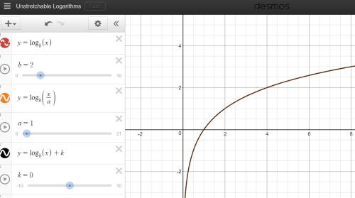
Any horizontal stretch of any logarithmic function is congruent to some vertical translation of the original function.  But for logarithms, vertical stretches do morph the curve into a different shape.  Here’s a Desmos page demonstrating the log property.

The sum property of logarithms proves the existence of this equally strange property:

CONCLUSION

Hopefully the unexpected transformational congruences will spark some nice discussions, while the graphical/algebraic equivalences will reinforce the importance of understanding mathematics more than one way.

Enjoy the strange transformational world of exponential and log functions!